Excel

1.How to create the Table

         1.Open a workbook (spreadsheet) or have one already open.

 2.Select a range of cells, if you wish. If you have already determined which cells will      make up your table, you can select that range of cells now. You can change this range later when you create the table.

3.Create the table.

• To create a list (table) in Excel 2003, select "List" from the Data menu.
• To create a table in Excel 2007 or 2010, select the range of empty cells or cells containing data that you want to have in your table. Then, either select "Table" from the Tables group on the Insert menu ribbon or select "Format as Table" in the Styles group on the Home menu ribbon, and select one of the table styles. (The former option applies Excel's default table style, while the other lets you choose a style when you create the table. You can later apply or change the table style by selecting one of the options from the Table Styles group in the Table Tools Design menu ribbon.)

  

     

4.Provide a data source for your table, if you did not previously select a group of cells. After you perform the appropriate action from those listed in the previous step for creating a data table or list table, a dialog box will appear, either the Create Table dialog (Create List dialog in Excel 2003) or the Format As Table dialog. The "Where is the data for your table?" field displays the absolute reference(s) for the current cell(s) selected. If you want to change this information, you can type in a different cell or range reference.

5.Indicate whether your table has headers. If your table has headers, check the "My table 
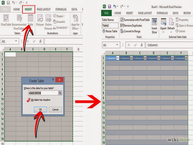
   has headers" box.

• If you don't check this box, the table will display default header names ("Column 1," "Column 2," etc.). You can change a column name by selecting the header and typing in your own name in the formula bar.

2.Give example for mathematics formula using Excel:-

This calculator will use cells A5 and B5 as the parameters and will show the addition, subtraction, division and multiplication results for those two numbers.

We'll start with the just the two parameters:

Then we can add the formula for the addition result:

You can see that when we change the parameters (A1,A2), the result of the addition formula for our mini calculator changes:

MISSING IMAGE?!

Let's now add the subtraction formula:

And again, when we change the parameters (A1,A2) the result changes.

Now let's flex your formula muscles...

Get a pen and a paper

Write down the multiplication and division formulas for our little Excel calclulator

Fire up Excel

Open a new sheet

Recreate the calculator (including the multiplication and division formulas)

                                                

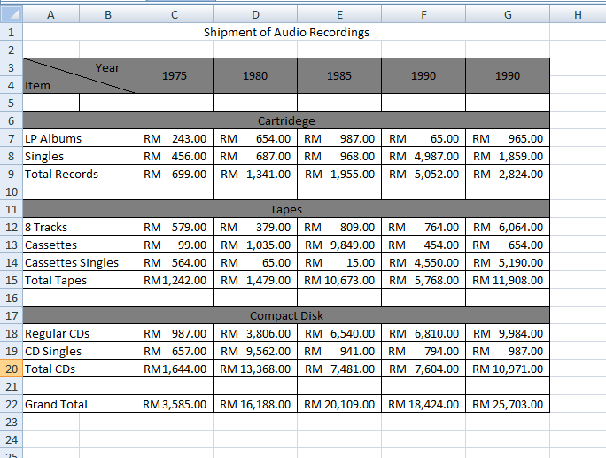
                                                3.How to insert Symbol RM with 2 decimal places.

Follow the steps bellows to insert MYR into the system :

Login to the admin panel

Goto System -> Localisation -> Currencies

Click [Insert] to add new currency to the system

Enter these value

Code : MYR

Symbol Left : RM

Symbol Right : - leave blank -

Decimal Places : 2

Value : - see note below-

Status : Enabled

Click [Save] when done

Now you can see "RM" symbol added to the currency option at your store front.

Notes :

1. How to set the value.

Go to Yahoo Currency Converter (you can search with Google)

Check the value of MYR compare to USD $1.

Set this value as the value in the currency setting above.

2. I prefer to set USD as the default currency.

3. OpenCart able to link to Yahoo Currency Converter to auto update the currency value from time to time.

4. You can actually do the same steps for any other currency.

conclusion

                                   i have learn how to use excel and its help me with the calculation and more.